Visualizing Model Comparison

When training deep neural networks, we often strive to compare the models and understand the consequences of different design choices beyond their final performance. We want to be able to explain different qualitative aspects of the solutions our models learn. To understand the solution a model converges to, we could either look into its parameter space or its representational space.

Sometimes, we can also gain some insights about how a model works by looking at its parameter values. For example, the weights of a linear classifier indicate which parts of input features are important for the models’ decision. Or in some cases it can be useful to track the changes in the parameter values during training, for example to visualize the optimizer trajectory of a model (Li et al., 2018).

For example, it can be very insightful to visualize the internal representations of the models in 2D or 3D using dimensionality reduction techniques such as PCA or t-SNE. This way, we are looking at the solutions from the representational aspect.

Now, let’s see how we can compare the solutions learned by multiple different models. Instead of visualizing how the weight of a single model look like or how one model represents different examples, we want to visualize a set of different models in a shared space so that we can directly see how they are compared to one another, i.e., we want to embed different models in a shared space. To do this, we need to measure the similarity between the models in some way.

Besides the performance of the models on a set of tasks, we can measure their similarity in terms of their parameters’ value or the way they represent different input examples.

Given multiple instances of the same model architecture, an obvious way to measure the similarity between them would be to compare the value of their parameters. However there are several flaws for this approach:

1. It is only applicable when the given models have exactly the same architecture, i.e., their parameter spaces are comparable.
2. The parameter space of the models can be very large and the simple approaches for computing distances would not be necessarily meaningful. Hence, we need to deal with the curse of dimensionality.

Another approach for comparing a set of models is to directly compare the representations we obtain from them. However, this is still only applicable if the representations from the given models are comparable and consequently have the same dimensionality. Moreover, this way, the similarity between the models will be sensitive to some trivial differences in the representational spaces of the models, e.g. if the representations obtained from model A are all a linear transformation of the representations obtained from model B, they are in principal 100% similar, but we can not capture this; if we are simply taking into account the similarities between the representations obtained for each individual example.

Fortunately, there are solutions that address all of the issues mentioned above, Representational Similarity Analysis (RSA) (Laakso & Cottrell, 2000) and Canocical Correlation Analysis (CCA) (Thompson, 1984).

RSA and CCA are standard tools of multivariate statistical analysis for quantifying the relation between two sets of variables. In our case, the sets of variable are the representations/embeddings of a set of examples obtained from each model. In CCA, to address the issue of having non comparable representational spaces, we first learn to map the representations from both models in a joint (low dimensional) space in a way that their correlation for each example is maximized. In RSA, instead of computing the similarity between representations, we compute the similarity of similarity of representations (second order similarity) in each space, thus we avoid the need to directly compare the representations from different spaces (obtained from different models).

So, if we have a set of models and we want to know how they are all compared to each other we can compute the representational similarity between each model pair using RSA or CCA (or some other similar technique). This will give us the similarity matrix of the models and we can visualize this in 2d or 3d using a multi dimensional scaling algorithm.

I will now explain how we can get the model embeddings within the RSA framework. In the figure below I have depicted the process of computing representational similarities between a sets of models using RSA.

Computing representational similarity of multiple models

Assume we have $m$ models, and we want to visualize them in 2d based on the similarity of the activations of their penultimate layers¹.

• First, we feed a sample set of size $n$ from the validation/test set (e.g. 1000 examples) to the forward pass of each model and obtain the representation from its penultimate layer (in fact, this can be any layer).
• Next, for each model, we calculate the similarity of the representations of all pairs from the sample set using some similarity metric, e.g., dot product. This leads to $m$ matrices of size $n\times n$ (part 1 in the figure above).
• We use the samples similarity matrix associated with each model to compute the similarity between all pairs of models. To do this, we compute the dot product (we can use any other measure of similarity as well) of the corresponding rows of these two matrices after normalization, and average all the similarity of all rows, which leads to a single scalar (part 2 and 3 in the figure above).
• Given all possible pairs of models, we then have a model similarity matrix of size $m\times m$ and we apply a multi dimensional scaling algorithm to embed all the models in a 2D space based on their similarities.

In the example below we see the similarity between the penultimate layers of the models trained on the MNIST dataset.

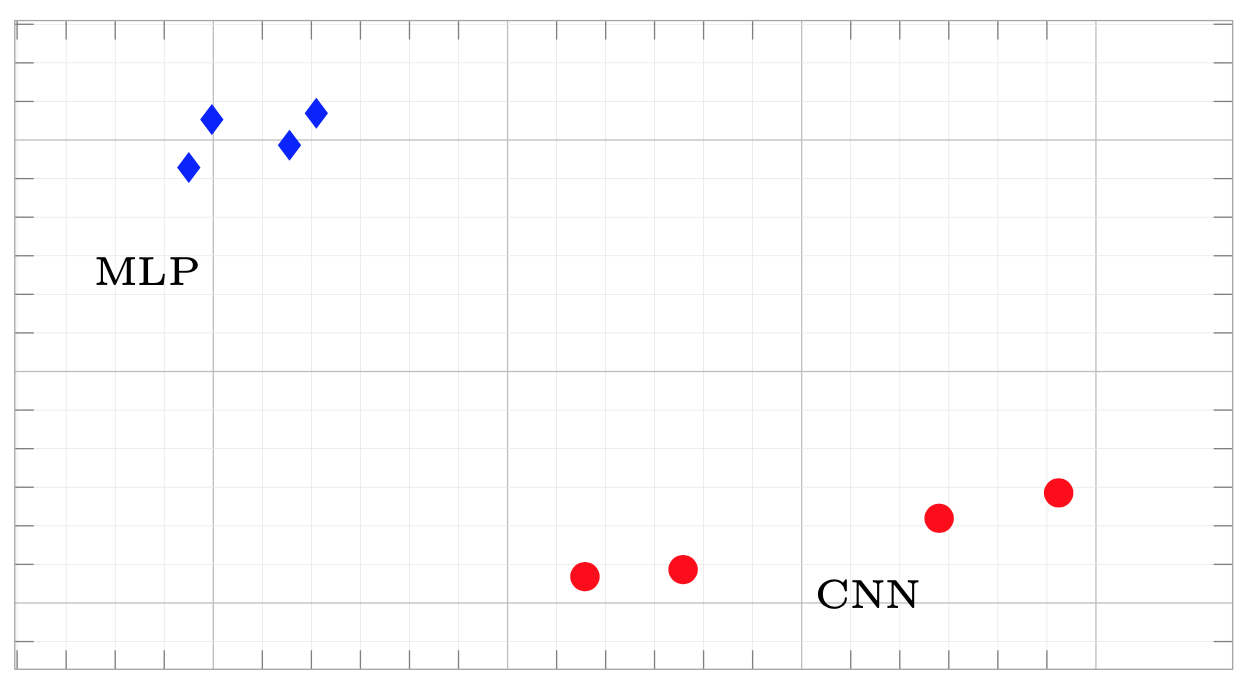
Representational similarity of different instances of MLPs and CNNs trained on MNIST

We can use this technique not only to compare different models but also to compare different components of the same model, e.g., different layers, or to see how the representations of a model change/evolve during training. For example, in figure below, we can see the training trajectories of a CNN and an MLP on the MNIST dataset. To obtain these training trajectories, we compute the pairwise similarity between the representations obtained from the models at different stages of the training process (different epochs).

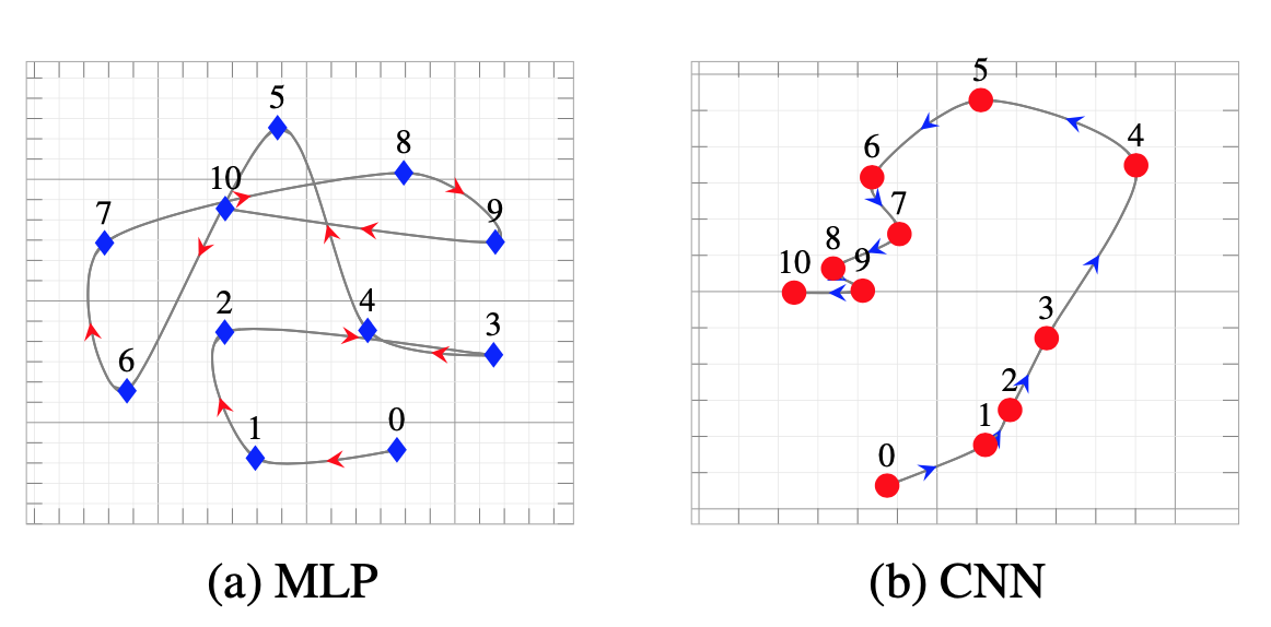
Visualizing training paths of models using RSA

When applying RSA, there three important factors that can affect the results:

1. The similarity metric used to compute the similarity between examples for each model.
2. The similarity metric used to compute the similarity between models, i.e., between the rows of the similarity matrices of the models).
3. The sets of examples used int the analysis.

We need to carefully choose the similarity metrics based on the nature of the representational spaces we are studying and our definition of similar representational spaces, e.g. do we want our measure to be sensitive to scales or not. And for the set of examples, we need to make sure that they are representative of the dataset.

RSA and CCA are very common techniques especially in the fields of computational psychology and neuroscience. In the recent years, they have also gained back their popularity in the machine learning community as methods of model analysis and interpretation.

If you are interested to sea how this can be used in practice, see our papers “Blackbox meets blackbox: Representational Similarity and Stability Analysis of Neural Language Models and Brains”, where we propose using RSA to measure stability of representational spaces of models against different factors, e.g. context length or context type for language models and “Transferring Inductive Biases through Knowledge Distillation”, where we use the techniques explained in this post to compare models with different architectures and inductive biases.

If you find this post useful and you ended up using this technique in your research please consider citing our paper:

@article{abnar2020transferring,
    title={Transferring Inductive Biases through Knowledge Distillation},
    author={Samira Abnar and Mostafa Dehghani and Willem Zuidema},
    year={2020},
    eprint={2006.00555},
    archivePrefix={arXiv},
}