No free lunch theorem states that for any learning algorithm, any improvement on performance over one class of problems is balanced out by a decrease in the performance over another class (Wolpert & Macready, 1997). In other words, there is no “one size fits all” learning algorithm.
We can see this in practice in the deep learning world. Among the various neural network architectures, each of them are better or worse for solving different tasks based on their inductive biases. For example, consider the image classification problem. CNNs are the de facto choice for processing images and in general data with grid-like topology. Sparse connectivity and parameter sharing in CNNs make them an effective and statistically efficient architecture.
The convolution operation in combination with max pooling makes CNNs approximately invariant to translation. When a module is translation invariant, it means that if we apply translation transformation on the input image, i.e., change the position of the objects in the input, the output of the module won’t change. In mathematical terms if is translation invariant, then , where is a translation function. A module could also be translation equivariant, which means that any translation in the input will be reflected in the output. In mathematical terms, if is translation equivariant, then . The convolution operation is translation equivariant, and applying a pooling operation on top of it results in translation invariance!
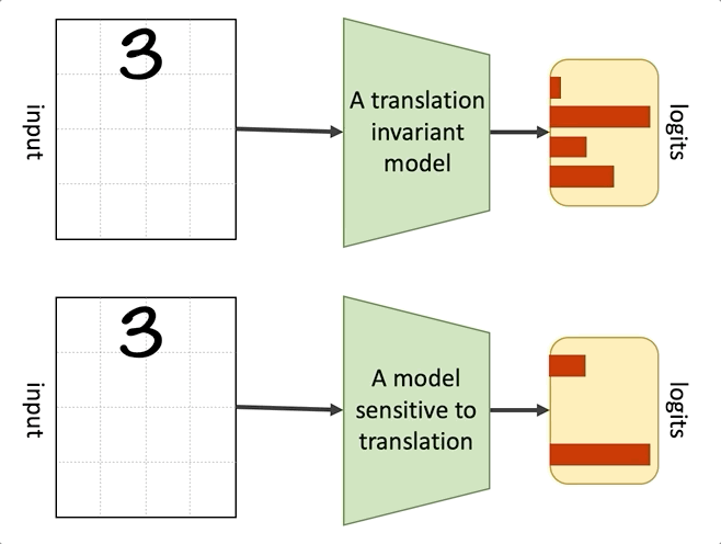
Translation invariance
Translation invariance of CNNs improves their generalization and makes them data efficient compared to fully connected networks. For example, if, during training, a CNN has only seen pictures of cats where the cat is located at the centre of the image, it can correctly classify cats at test time independent of their position in the image. In the lack of this inductive bias, the model needs to see examples of cats at different positions to be able to correctly classify them at test time. On the other hand, this translation invariance can hurt the performance of CNNs in cases where the position of the objects in the image matters. This is known as the Picasso effect, where you have all the pieces of an object but not in the right context (One of the motivations behind CapsNets is to address this drawback).
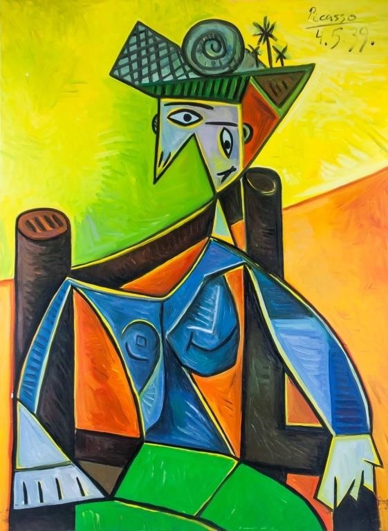
Oil on canvas, featuring a cubist portrait, attributed to Pablo Picasso (1881-1973, Spanish)
Another example of such tradeoffs are recurrent neural networks (RNNs) in contrast to Transformers. It has been shown that the recurrent inductive bias of RNNs helps them capture hierarchical structures in sequences (Take a look at my other blog post about the recurrecnt inductive bias). But this recurrence and the fact that RNNs’ access to previous tokens is limited to their memory makes it harder for them to deal with long term dependencies. Besides, RNNs can be rather slow because they have to process data sequentially, i.e, they are not parallelizable. On the other hand, Transformers have direct access to all input tokens and they are very expressive when it comes to representing longer context sizes. Also, they can process the input sequence in parallel, hence they can be remarkably faster than LSTMs. However, Transformers struggle to generalize on tasks that require capturing hierarchical structures when training data is limited.
It might not be possible to have one model that can single handedly achieve the desired generalization behaviour on a wide range of tasks, but would it be possible to benefit from the inductive biases of different models during training to have one best model at inference?
Fortunately, it seems to be possible to do this to some extent! In this post, I discuss our paper, “Transferring Inductive Biases through Knowledge Distillation”, where we show that it is possible to transfer the effect of inductive bias through knowledge distillation and this can be a step toward achieving the goal of combining the strengths of multiple models in one place.
What is Inductive bias?
Inductive biases are the characteristics of learning algorithms that influence their generalization behaviour, independent of data. They are one of the main driving forces to push learning algorithms toward particular solutions (Mitchell, 1980). In the absence of strong inductive biases, a model can be equally attracted to several local minima on the loss surface; and the converged solution can be arbitrarily affected by random variations, for instance, the initial state or the order of training examples (Sutskever et al., 2013; McCoy et al., 2020; Dodge et al., 2020).
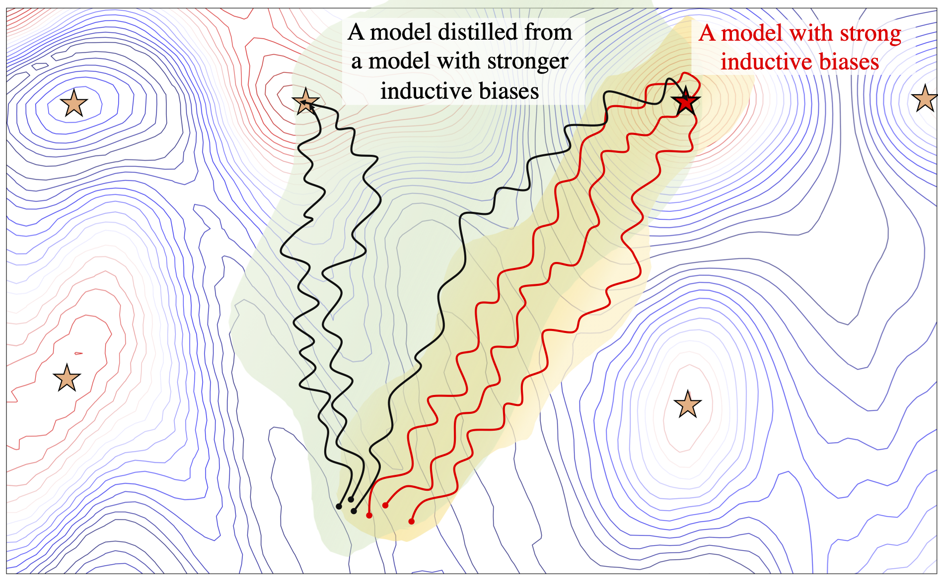
In figure below, we see a schematic example of the paths that different instances of two models with different levels of inductive biases follow on a fitness landscape.1
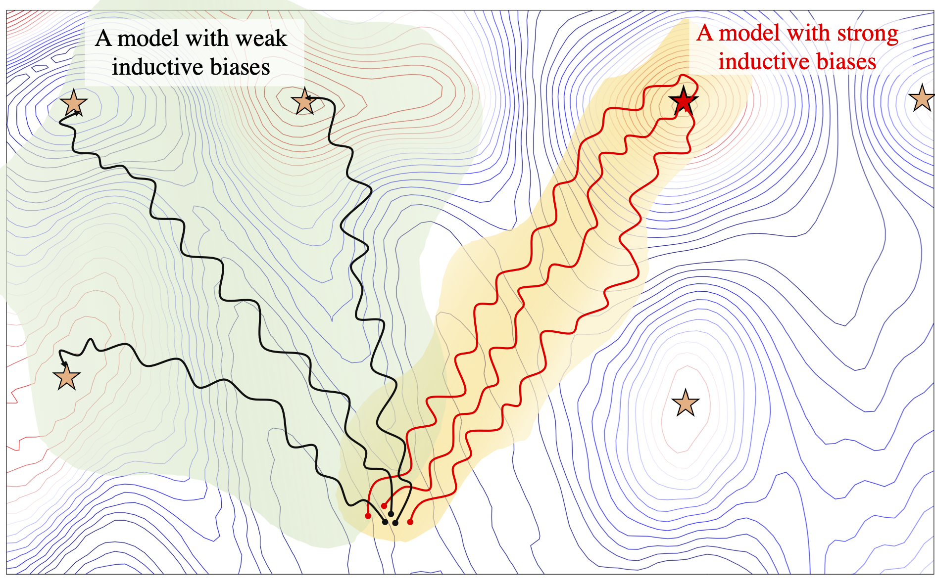
A drawing of how inductive biases can affect models' preferences to converge to different local minima. The inductive biases are shown by colored regions (green and yellow) which indicates regions that models prefer to explore.
There are two types of inductive biases: restricted hypothesis space bias and preference bias. Restricted hypothesis space bias determines the expressively of a model, while preference bias weighs the solutions within the hypothesis space (Craven, 1996).
From another point of view, as formulated by (Seung et al., 1991) we can study models from two aspects:
- Whether a solution is realisable for the model, i.e., there is at least one set of weights that leads to the optimal solution.
- Whether a solution is learnable for the model, i.e., it is possible for the model to learn that solution within a reasonable amount of time and computations.
In many cases in deep learning, we are dealing with models that have enough expressive power to solve our problems, however, they have different preference biases. Meaning the desired solutions are realisable for all of them, but depending on the task at hand it is more easier for some of them to learn the solutions compared to the others.
Having the Right Inductive Bias Matters
To understand the effect of inductive biases of a model, we need to take a look at its generalization behaviour.
Let’s walk through the example of LSTMs and Transformers. When we train these models on language modelling, i.e., predicting the next word in a sequence, they both achieve more or less similar perplexities. But how can we know which one is learning a more generlizable solution? One way to check the generalizability of language models is to test how well they have learned the syntactic rules of the language and the hierarchical structures of the sentences. The task of subject-verb agreement is designed for this purpose, i.e., to assess the ability of models to caputre hierchical structure in the language. In this task, the goal for the model is to predict the number of a masked verb in a given sentence. To do this, the model needs to correctly recognize the subject of the verb in the sentence and the main difficulty is when the verb does not follow the subject immediately and there are one or more agreement attractors2 between the subject and the verb. In the figure below, we see an example for this task.
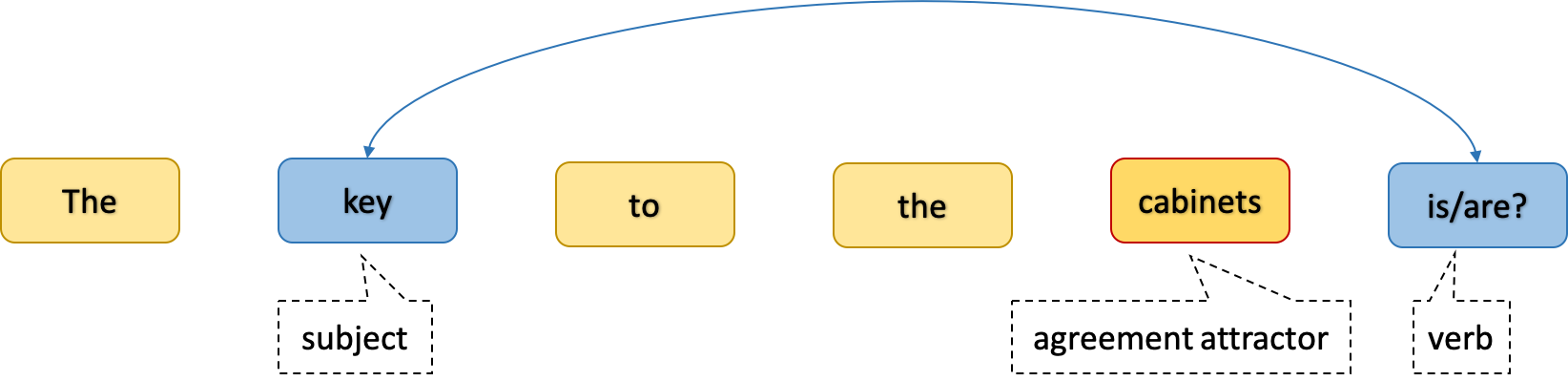
An example from the subject-verb agreement task
Comparing different instances of LSTMs and Transformers, with different perplexities, we observe that LSTMs have a higher tendency toward solutions that achieve better accuracy on the subject verb agreement task. We can see that, LSTMs with worse perplexities achieve better accuracies than Transformers with better perplexities.
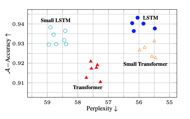
Accuracy on verb number prediction vs perplexity
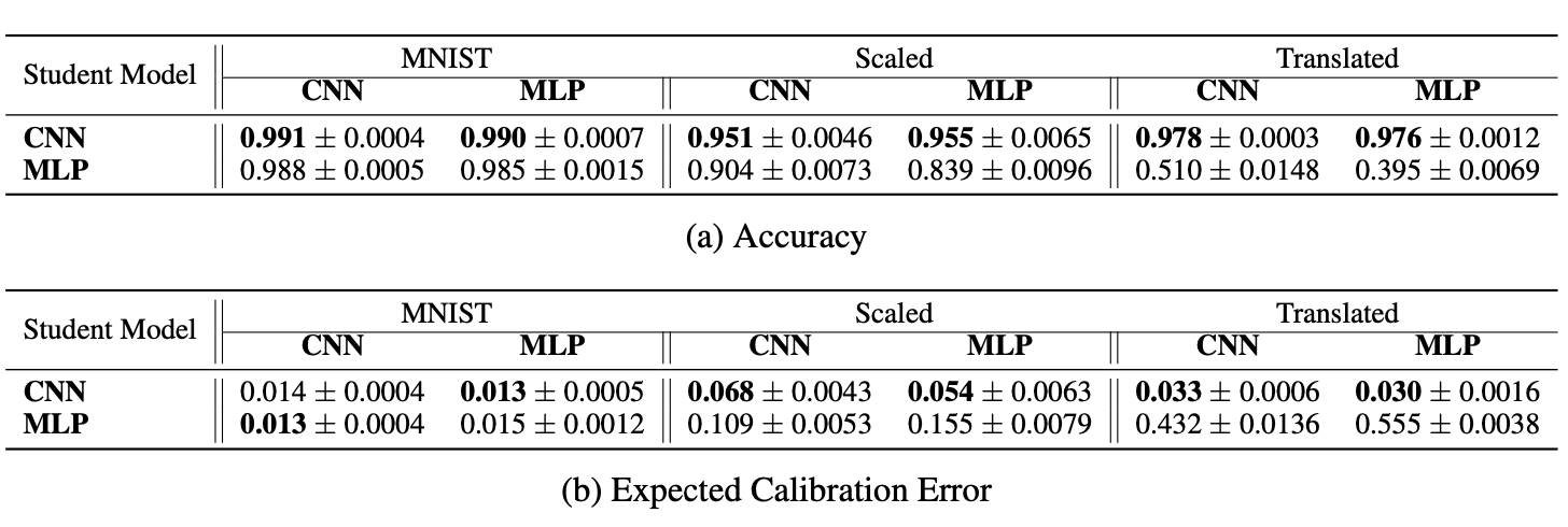
Now, let’s go back to the CNN example and see how the inductive bias of CNNs works in practice. We can view CNNs as MLPs with an infinitely strong prior over their weights, which says that the weights for one hidden unit must be identical to the weights of its neighbor but shifted in space, also that the weights must be zero, except for in the small, spatially contiguous receptive field assigned to that hidden unit (Goodfellow et al., 2016). Hence, to measure the effectiveness of the CNNs inductive biases we can compare them to MLPs. Here you can see the results of training CNNs and MLPs on the MNIST dataset and evaluating them on the translated and scaled version of MNIST from the MNIST-C dataset.
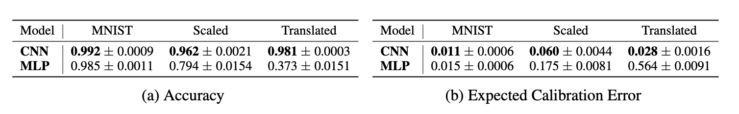
Accuracy and Expected Calibration Error (mean$\pm$std over multiple trials) of CNNs and MLPs trained on MNIST and evaluated on MNIST, MNIST-Scaled and MNIST-Translated
As expected, even though the accuracies of MLPs and CNNs are only slightly different on the original MNIST test set, CNNs can generalize much better to the out of distribution test sets that include translated and scaled MNIST examples.
Knowledge Distillation to the Rescue
There are different ways to inject inductive biases into learning algorithms, for instance, through architectural choices, the objective function, curriculum strategy, or the optimisation regime. Here, we exploit the power of Knowledge Distillation (KD) to transfer the effect of inductive biases between neural networks.
A drawing of how inductive biases can be transferred through distillation. The inductive biases are shown by colored regions (green and yellow) which indicates regions that models prefer to explore.
KD refers to the process of transferring knowledge from a teacher model to a student model, where the logits from the teacher are used to train the student. It is best known as an effective method for model compression (Hinton et al., 2015) which allows taking advantage of the huge number of parameters during training, without losing the efficiency of a smaller model during inference. When we have a teacher that performs very well on a given task, using it to train another model can lead to an improved performance in the student model. The question is where does this improvement come from. Does knowledge distillation merely act as a regularization technique or are the qualitative aspects of the solution the teachers converges to that are rooted in its inductive biases, also reflected in the student model.
Interestingly, the improvement we get from KD is not limited to the performance of the model on the trained task. Through distillation, the generalization behaviour of the teacher that is affected by its inductive biases also transfers to the student model.
In the language modelling example, even in the case where the perplexity increases (worsens), the accuracy on the subject verb agreement task improves.
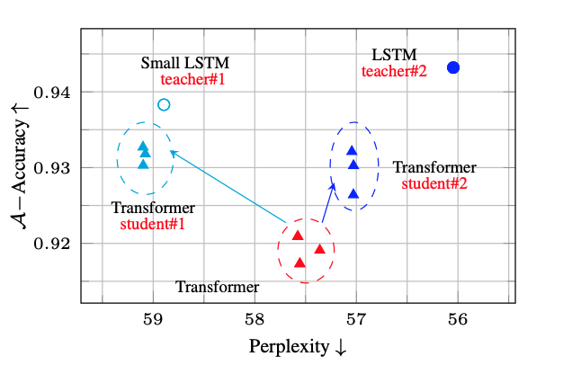
Changes in accuracy vs perplexity through distillation
In the MNIST example, not only the performance of the student model on the MNIST test set improves, it also achieves higher accuracies on the out of distribution sets.
Performances of CNNs and MLPs trained through distillation
Distillation affects the trajectories the student models follow during training
Now, Let’s take a look at the training paths of the models when they are trained independently and when they are trained through distillation. Figure below shows the training path for an independent MLP, an independent CNN, and an MLP that is distilled form a CNN (To learn more about the details of how we made this visualizations see my other blog post). We see that while MLP and CNN seem to have very different behaviour during training, the student MLP with a CNN as its teacher behaves differently than an independent MLP and more similar to its teacher CNN. This is interesting, in particular, since the student model is only exposed to the final solution the teacher has converged to and no information about the intermediate stages of training is provided in the offline KD.
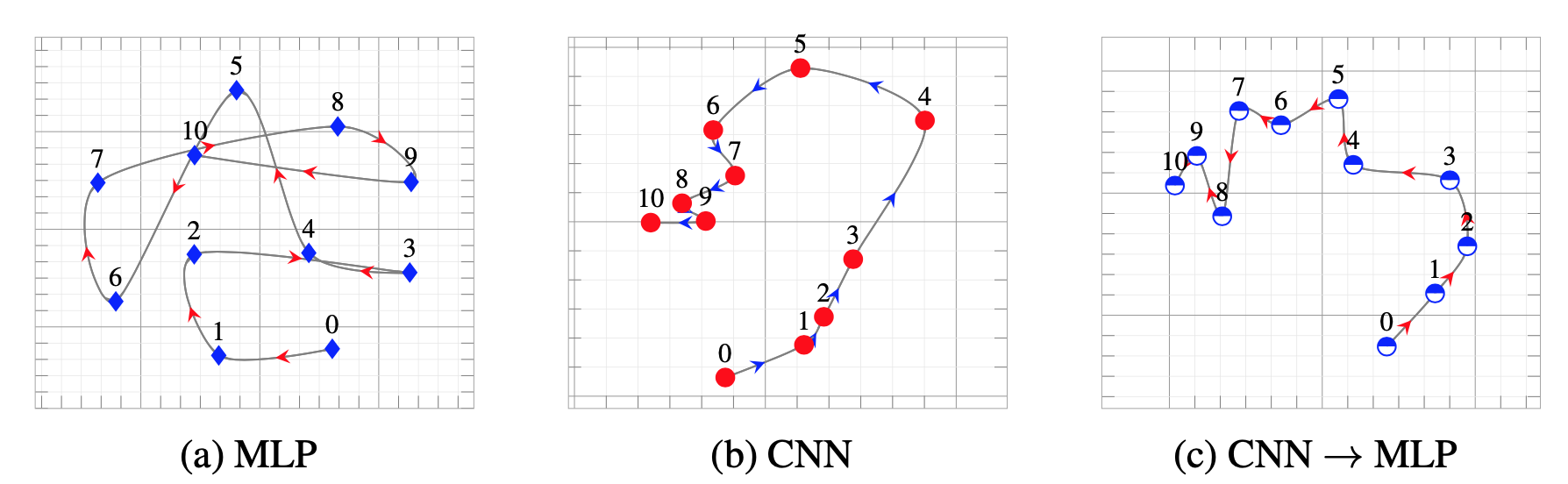
Training paths of CNNs and MLPs
Moreover comparing the final representations these models converge to, we see that as expected based on our assumptions about the inductive biases of these models, MLPs have more variance than CNNs, and Transformers have more variance compared to LSTMs. Also, distillation from a teacher with stronger inducive biases results in representations that are more similar to the representations learned by the teacher model. Finally, self-distillation does not significantly change the representations the models learn.
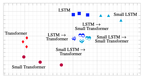
Representational similarity of converged solutions of LSTMs and Transformers
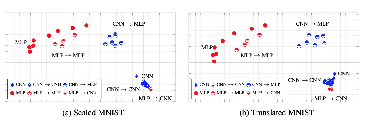
Representational similarity of converged solutions of CNNs and MLPs
Where else can this be usefull?
Here our focus is on the generalizability of the solutions learning algorithms converged to, but this analysis can be potentially extended to other types of biases, e.g., biases that would trigger ethical issues. Considering the fact that knowledge distillation is a very popular model compression technique, it is important that we understand the extent to which different types of biases can be transferred from one learning algorithm to another through knowledge distillation.
In this post, I went through the findings of our paper on “Transferring Inductive Biases Through Knowledge Distillation”, where we explore the power of knowledge distillation for transferring the effect of inductive biases from one model to another.
Codes to replicate the experiments we discussed in this post are available here.
If you find this post useful and you ended up using our code in your research please consider citing our paper:
@article{abnar2020transferring,
    title={Transferring Inductive Biases through Knowledge Distillation},
    author={Samira Abnar and Mostafa Dehghani and Willem Zuidema},
    year={2020},
    eprint={2006.00555},
    archivePrefix={arXiv},
}