Special thanks to Sara Sabour and Mostafa Dehghani for their valuable feedback on the content of this post!
In this post, we go through the main building blocks of transformers (Vaswani et al., 2017) and capsule networks (Hinton et al., 2018) and try to draw a connection between different components of these two models. Our main goal here is to understand if these models are inherently different, and if not, how they relate.
Transformers, or so-called self-attention networks, are a family of deep neural network architectures, where self-attention layers are stacked on top of each other to learn contextualized representations for input tokens via multiple transformations. These models have been able to achieve SOTA on many vision and NLP tasks. There are many implementation details about the transformer. Still, at a high level, transformer is an encoder-decoder architecture, where each of encoder and decoder blocks consists of a stack of transformer layers. In each layer, we learn to (re-)calculate a representation per input token. This representation is computed by attending to the representations of all tokens from the previous layer. This is illustrated in the figure below.
![]()
Thus, to compute the representations in layer $L+1$, the representations from the lower layer, $L$, are passed through a self-attention block, which updates the representation of every token with respect to all the other tokens. The future tokens are masked in the self-attention in the decoder block. Also, besides the self-attention, there is encoder-decoder-attention in the decoder (which is not depicted in the figure above). To see more details about the transformer, check out this great post: http://jalammar.github.io/illustrated-transformer.
The main component of transformer is the self-attention, and one essential property of it is using a multi-headed attention mechanism. In this post, we mainly focus on this component and dig into some of its details as we get back to it when comparing capsule nets with transformers.
The primary motivation of using multi-head attention is to get the chance of exploring multiple representation subspaces since each attention head gets a different projection of the representations. In an ideal case, each head would learn to attend to different parts of the input by taking a different aspect into account, and it is shown that in practice, different attention heads compute different attention distributions. Having multiple attention heads in transformers can be considered similar to having multiple filters in CNNs.
Here, we explain how information from different positions in a lower layer, $L$, are integrated using multi-head self-attention, to compute the higher layer, $L+1$ representations.
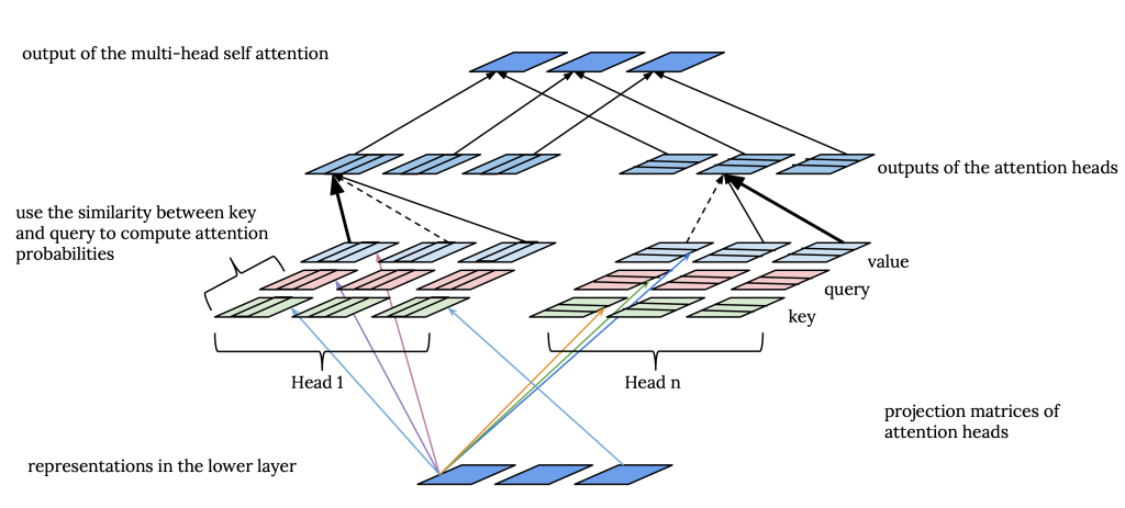 First of all, we should note that the representations for each position at each layer are seen as (key, value, query) triplets. Thus, for each layer, we have three matrices (K, Q, V), where each row in these matrices corresponds to a position.
The input to attention head $i$ is a linear transformation of the K, Q and V: $K_i = W_k^{i}K$, $V_i = W_v^{i}V$, $Q_i = W_q^{i}Q$
And, the output of attention head $i$ is:
where $d_i$ is the length of $K_i$.
Intuitively speaking, the representation of each position in layer $L+1$, is a weighted combination of all the representations in layer $L$. In order to compute these weights, the attention distributions, each attention head, computes the similarity between the query in each position in layer $L+1$ to the keys of all positions in layer $L$. Then, the distribution of attention over all positions is computed by applying the softmax function on these similarity scores. Thus, for each position in each self-attention layer, we have a distribution of attention weights over the positions in the lower layer per attention head. Eventually, for each attention head, the values at all positions are combined using the attention probabilities of the head. In the last step, the values of all the attention heads are concatenated and transformed linearly to compute the output of the multiple head attention component:
So, in terms of the parameters that are learned, for each layer, we have one transformation matrix, $W_o$, which is applied on the concatenation of the outputs from all the attention heads, and we have a set of three transformation matrices for each attention head, i.e. $W^i_k$, $W^i_q$, and $W^i_v$.
Matrix Capsules with EM routing:
Capsule networks, in the first place, were proposed to processes images in a more natural way. In 2000, Hinton and Ghahramani argued that the image recognition systems which rely on a separate preprocessing stage suffer from the fact that the segmenter does not know the general information about the object and propose to have a system in which recognition and segmentation are done simultaneously (Hinton et al., 2000). The idea is that in order to recognize parts (segments) of an object, you need to first have a general understanding of what the object is. In other words, we need to have both top-down and bottom-up flow of information. This can also be true for NLP problems. An example of this is parsing garden path sentences. Capsule networks can be viewed as a CNN, where there is some structure on the outputs of the kernels and pooling is replaced by dynamic routing.
A capsule is a unit that learns to detect an implicitly defined entity over a limited domain of viewing conditions. It outputs both the probability that the entity is present and a set of “instantiation parameters” that reflect the features of the entity such as pose information. The presence probability is viewpoint invariant, e.g. it does not change as the entity moves or rotates, whereas the instantiation parameters are viewpoint equivariant, e.g. they change if the entity moves or rotates.
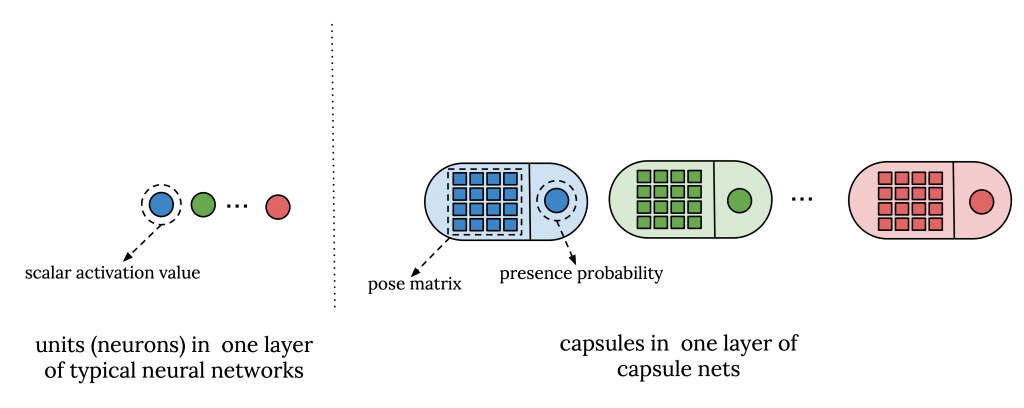 In matrix capsules with EM routing, they use a capsule network that includes a standard convolutional layer, and a layer of primary capsules followed by several layers of convolutional capsules. In this version of the capsule net, the instantiation parameters are represented as a matrix called the pose matrix.
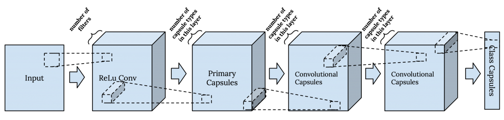 Each capsule layer has a fixed number of capsule types (similar to filters in CNNs), which is chosen as a hyper-parameter. A capsule is an instance of a capsule type. Each capsule type is meant to correspond to an entity, and all capsules of the same type are extracting the same entity at different positions. In lower layers, capsule types learn to recognize low-level entities, e.g. eyes, and in higher layers, they are supposed to present more high-level entities, e.g. faces.
In the convolutional capsule layers, the weight matrix of each capsule type is convolved over the input, similar to how kernels are applied in CNNs. This results in different instances of each capsule type.
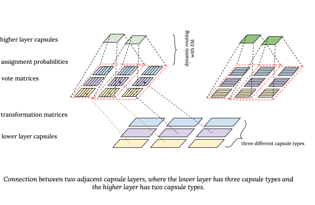 In capsule nets, the number of capsule types in each layer is predefined. Between every capsule type in two adjacent layers, there is a transformation matrix. This way, each higher layer capsule, sees the entity in the lower layer capsule from a different point of view.
The Pose Matrix
This equation shows how the pose matrix of a higher layer capsule, $M_j$, is computed based on the pose matrix of lower layer capsules, i.e $M_i$s:
In this equation, $r_{ij}$ is the assignment probability of $capsule_i$ to $capsule_j$, or in other words, how much $capsule_i$ contributes to the concept captured by $capsule_j$. $W_{ij}M_i$ is the projection of the pose matrix of the lower layer $capsule_i$ with respect to $capsule_j$, which is also called the “vote matrix”, $V_{ij}$. So, the pose matrix of $capsule_j$ is basically a weighted average of the vote matrices of the lower layer capsules. Note that the assignment probabilities are computed as part of the EM process for dynamic routing and are different from the presence probability or activations probability of the capsules.
The Presence Probability
Now, let’s see how the activation probabilities of the higher layer capsules are computed. In simple terms, the activation probability of a capsule in the higher layer is computed based on the cost of activating it versus the cost of not activating it.
The question is, what are these costs, and how do we compute them?
If the sum of the assignment probabilities to a higher layer capsule is more than zero, i.e. there are some lower layer capsules assigned to this capsule, there is a cost for not activating that capsule. But the activation probability of a capsule is not calculated only based on the values of the assignment probabilities. We should also consider how well the vote matrices of the lower layer capsules assigned to the higher layer capsule are consistent with each other.
In other words, the lower layer capsules assigned to the higher layer capsule should be part of the same entity that the higher layer capsule is representing. So the cost for activating a capsule also reflects the level of inconsistencies between the vote matrices of the lower layer capsule and the pose matrix computed for the higher layer capsule. In addition, to avoid trivially activated capsules, there is a fixed penalty for activating each capsule.
Dynamic Routing with EM
The main challenge here is to compute assignment probabilities, $r_{ij}$. This basically means how to connect the lower layer capsules, $\Omega_L$, to the higher layer capsules $\Omega_{L+1}$, or in other words, how to route information between capsule layers. We want these connections to not only depend on the presence of the lower layer capsules but also based on their relevance to each other as well as to the higher layer capsule. For example, a capsule representing an eye, which is part of a face, probably should not be connected to a capsule which represents a table. This can be seen as computing the attention from the lower layer capsules to the higher layer capsules. The problem is, we have no initial representation for the higher-level capsules in advance to be able to calculate this probability based on the similarity of the lower layer capsule with the higher layer capsule. This is because the representation of a capsule depends on which capsules from the lower layer are going to be assigned to it. This is where dynamic routing kicks in and solves the problem by using EM.
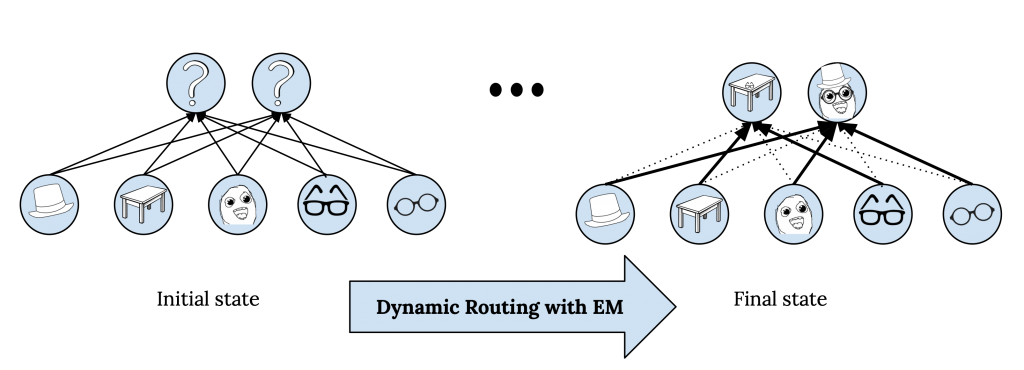 We can use EM to compute representations of $\Omega_{L+1}$ based on the representations of $\Omega_L$ and the assignment probabilities of the lower layer capsules to the higher layer capsules. This iterative process is called dynamic routing with EM. Note that dynamic routing with EM is part of the forward pass in Capsule Nets, and during training, the error is back-propagated through the unrolled iterations of dynamic routing.
It is noteworthy that, the computations are a bit different for the primary capsule layers since the layer below them is not a capsule layer. The pose matrices for the primary capsules is simply a linear transformation of the outputs of the lower layer kernels, and their activation is the sigmoid of the weighted sum of the same set of lower-layer kernel outputs. In addition, the final capsule layer has one capsule per output class. When connecting the last convolutional capsule layer to the final layer, the transformation matrices are shared over different positions, and they use a technique called “Coordinate Addition” to keep the information about the location of the convolutional capsules.
Capsule Nets vs Transformers:
Finally, we get to the most exciting part to compare these two models. While from the implementation perspective, capsule Nets and transformer don’t seem to be very similar, there are a couple of functional similarities between the different components of these two families of models.
Dynamic Routing vs Attention
In capsule networks, we use dynamic routing to determine the connection from the lower layer to the higher layer, in par with this in transformers we employ self-attention to decide how to attend to different parts of the input and how information from different parts contribute to the updates of representations. We can map the attention weights in transformer to assignment probabilities in capsule net; however, in capsule nets, the assignment probabilities are computed bottom-up, whereas in transformer the attention is computed top-down. i.e. the attention weights in transformer are distributed over the representations in the lower layer, but in capsule nets, the assignment probabilities are distributed over the higher layer capsules. Note that, it is true that in transformer, the attention probabilities are computed based on the similarity of the representations in the same layer, but this is equivalent to the assumption that the higher layer is first initialized with the representations from the lower layer and then it is updated based on the attention probabilities computed by comparing these initial representations with the representations from the lower layer.
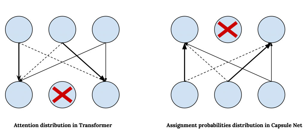 The bottom-up attention in capsule nets along with having a presence probability and the penalty for activating capsules, explicitly allows the model to abstract away the concepts as the information propagates to the higher layers. On the other hand, in transformer, the top-down attention mechanism allows the nodes in the higher layer not to attend to some of the nodes in the lower layer and filter out the information that is captured in those nodes.
Now, the question is, why do we need EM for dynamic routing in capsule nets? Why can’t we use a similar mechanism used to compute attentions in transformer to calculate assignment probabilities in capsule nets?
Presumably, we could use dot product similarity to compute the similarity of a lower layer capsule with the higher layer capsules to compute the assignment probabilities.
The challenge is that in capsule nets, we don’t have any prior assumption on the representations of the higher layer capsules since what they are supposed to represent are not known in advance. On the other hand in transformer the number of nodes in all layers are the same and equal to the number of input tokens, thus we can interpret each node as a contextualized representation of the corresponding input token. This let us initialize the representations in each higher layer with the corresponding representations from the lower layer, which allows us to use the similarities scores between the representations to compute the attention weights.
Capsule Types and Attention Heads:
Both capsule nets and transformer architectures have a mechanism which allows the models to process the representations from a lower layer from different perspectives to compute the representation in the higher layer. In capsule nets, there is a different transformation matrix between each pair of capsule types from two adjacent layers. Thus capsules that are instantiations of different capsule types view the capsules in the previous layer from a different point of view. In par with this, in transformer, we have multiple attention heads, where each attention head uses a different set of transformation matrices to compute the projection of key, value and query. So, each attention heads works on a different projection of the representations in the lower layer. Both these mechanisms serve a similar purpose as having different kernels in convolutional neural networks.
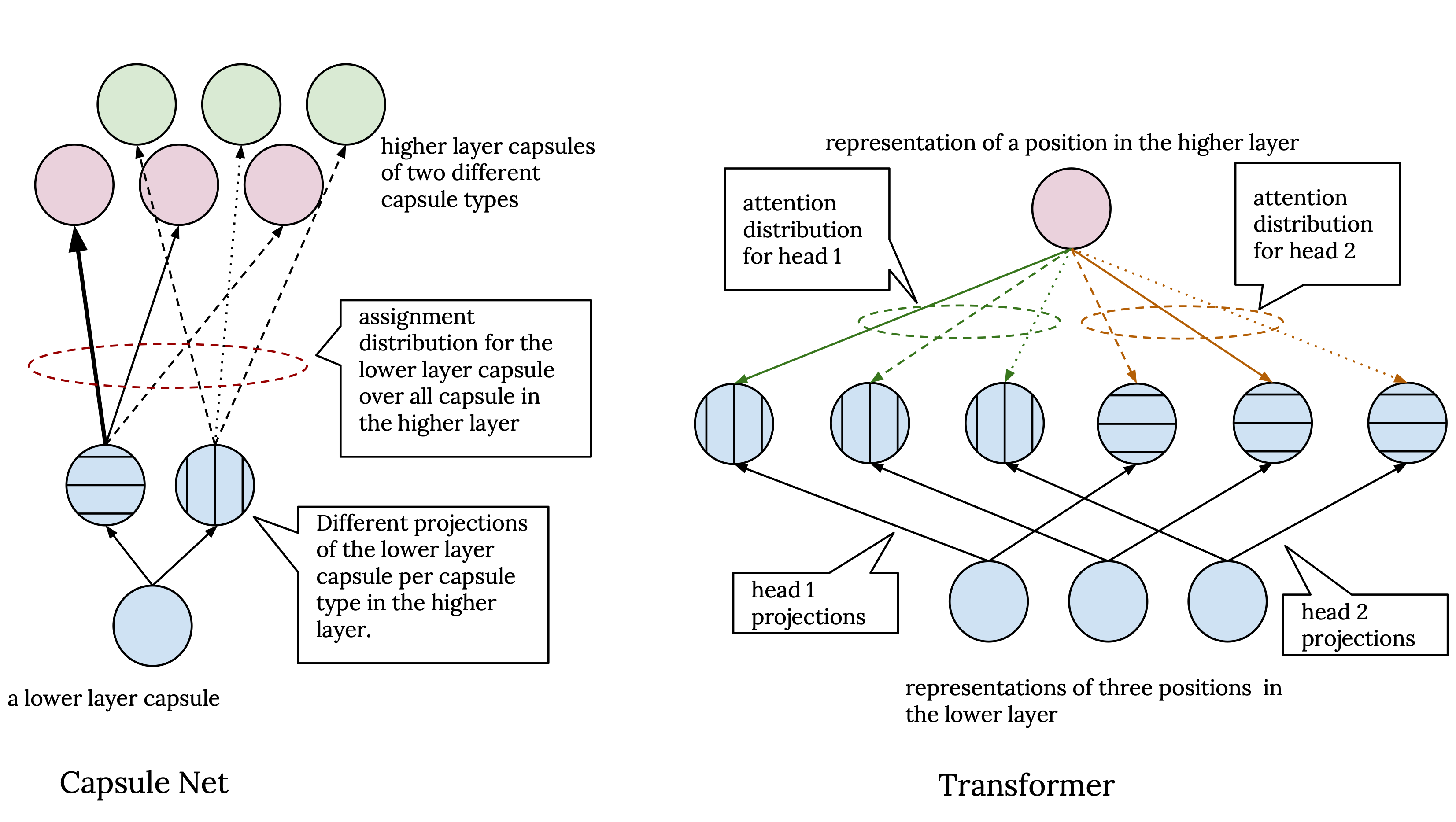 Now, what is different between capsule networks and transformers in this regard is that, in capsule networks, while capsules with different types have a different point of view, in the end, assignment probabilities for a capsule in the lower layer are normalized over all capsule in the higher layer regardless of their type. Hence we have one assignment distribution per each capsule in the lower layer. Whereas in transformer, each attention head independently processes its input. This means we have a separate attention distribution for each position in the higher layer, and the outputs of the attention heads are only combined in the last step, where they are simply concatenated and linearly transformed to compute the final output of the multi-headed attention block.
Positional embedding and coordinate addition:
In both transformer and capsule nets, there is some mechanism to explicitly add the position information of the features into the representations the models compute. However, in the transformer, this is done before the first layer, where the positional embeddings are added to the word embeddings. In contrast, in capsule nets, it is done in the final layer by coordinate addition, where the scaled coordinate (row, column) of the centre of the receptive field of each capsule is added to the first two elements of the right-hand column of its vote matrix.
Structured hidden representations:
In both transformer and capsule nets, the hidden representations are structured in some way. In capsule nets, instead of scalar activation units in standard neural networks, we have capsules where each one is represented by a pose matrix and an activation value. The pose matrix encodes the information about each capsule and is used in dynamic routing to compute the similarity between lower layer capsules and higher layer capsules, and the activation probability determines their presence/absence.
In par with this, in transformer, the representations are decomposed into key, query, and value triplets, where key and query are addressing vectors used to calculate the similarity between different parts of the input, and compute the attention distribution to find the extent to which different parts of the input contribute to each others’ representations.
In very loose terms, the pose matrix in capsule nets plays the role of key and query vectors in transformers. The main point here is that there seems to be some advantage in disentangling representations that are encoding different kinds of information. In both these models, this is done based on the roles of the hidden state in the routing or attention process.